Written by Ségolène Tarte

Thursday, 30 October 2008 17:57

In the last months, a large part of my efforts have been concentrated on extracting the strokes from the images of our texts. The good news is, I'm getting closer to actually extracting those strokes by the day!

In image processing terms, what I'm trying to do is perform feature extraction from the images. A number of methods are available, but our images are such, that we need to get away from traditional methods such as simple thresholding, or plain classical edges and corner detection (Canny edge detection, Hough transform, etc...) The reason for this is that our images are extremely noisy (i.e., a lot of information in the image is irrelevant information), and the classical methods don't work well on noisy images. There is one method though that has the potential to help us extract these features we're looking to extract. This method is the so-called phase congruency method [1]. And it's the one I've been working on. [ ... ]

1 The principle

The phase congruency method stems from signal processing. A signal (just like an image) is simply a function, that measures for example temperature as a function of time. If the temperature is measured very often, say every 0.1 second, throughout one day, then, due to measurement errors, instead of getting a nice smooth curve, we would get a curve that reflects also the variations in measurement errors, and the curve would look all jagged. However, the global tendency of the curve would show as expected, a bell-shaped curve during the day with a maximum around 1PM, solar time, and a minimum around 1AM solar time(!). Now imagine, the temperature is measured during 7 days. Well to study the resulting curve of actual measurements, a typical approach is to look at the frequencies. This means that instead of expressing the temperature as a function of time, we decide to describe our curve differently. The new description of the curve is made based on quantities called energy and phase as functions of frequencies, they do however describe as precisely the original curve as the temperature/time description, only in different terms. An operation called Fourier transform actually enables to switch freely back and forth from the temperature/time domain to the frequency/energy/phase domain (under certain mathematical assumptions of course, such as integrability of the temperature/time curve). And it is actually much easier to get rid of the jagged-ness of the curve when describing it in frequency/energy/phase than when describing it in time/temperature. And, pushing it further, it is also possible to look at the energy and phase values as functions of frequency at a given point on the original time/temperature curve; we then talk about local energy and local phase.

Well this whole principle can be applied to images too. An image is actually nothing more than a function of two variables, where instead of the one variable time, two variables describe a point in the image, a spatial point (x,y) located in a plane, and the value of the function at that point is the colour of the image at that point (in general, for grey level images, it's an integer value between 0 and 255). Now the same Fourier transform (adapted to the 2D domain, in contrast with the 1D time domain) can be applied, and a new description of the image can be made. We then describe our image in terms of energy, phase and direction (or orientation) as functions of frequency; in this 2D case, frequency is actually called scale, because it is a counterpart to a space measurement and not to a time measurement. And just as in the 1D case, we can also define local energy, local phase and local orientation for each point in the image (this is far from trivial, here, but I'll pass you the details! [2]).

Now, here is the sweet piece of "magic": it so happens that when a feature is present in the image at a point (x,y), then its local phase is constant throughout the scales [1,2,3].... So all I have to do in theory is to look for those points where the local phase is constant throughout the scales...

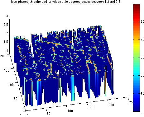
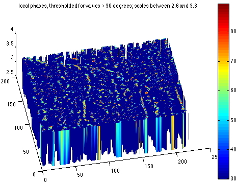
2 In practice

The principle sounds simple enough, doesn't it? Well in practice it gets tricky. It gets tricky, because computing the local phase for a range of scales is far from straight forward. In practice, we can only compute the local phase for a group of scales. So what happens is that we apply what are called "band-pass" filters to the image first, and then for each filtered image, we compute local phase, local orientation and local energy at every point. Then we need to look at the consistency of the local phase value throughout the filtered versions. The family of filters we use span a range of scales that can be assimilated to "fine grain" or "coarse grain"; with band-pass filters, we can choose to look at the image within a certain range of selected scales, so by choosing the "band-pass" appropriately we can look at the images within only a certain range of scales present in them. By moving the "band" of the band pass filter, we can span a larger range of scales separately. At this stage, a number of choices need to be made:

filters: The choice of the family of filters is crucial and tends to differ depending on the nature of the images [4].We are restricted by the fact that these filters need to be "band-pass" filters, yet that is a restriction that still leaves quite some room for manoeuvre (the "width" of the "band" and how many successive separate bands we look at). The three family of filters I am currently testing are the Mellor-Brady filters [5] (c.f., images below), the Difference Of Gaussians filters, and the log Gabor filters.
phase congruency: There is a standard way of computing phase congruency [3], but a quick look out our data shows that it wouldn't be appropriate here. The standard way of computing the phase congruency is based on the fact that when the local energy is high, we are more likely to trust the local phase value. Unfortunately, as our images are extremely noisy, the local energy is always relatively small, and although there are areas where it is high(ish!), these areas do not correspond to the areas where the feature information is valuable but rather to areas where the noise in the image peaks. We thus have to devise a new way of determining the consistency of the phase throughout scales. At this stage, I am actually thinking that there still is one piece of information that we haven't used and that is valuable, and it's the local orientation. We could use this to compute the standard deviation of the phase value throughout scales not just at a given point, but around a given point, where the shape of the "around" would be conditioned by the local orientation.

And as a bonus, our work on designing the Interpretation Support System is going to greatly facilitate our image processing job, using what we have called an elementary percept as an entity to process (see here for more details on the concept of elementary percept). Indeed the filtering and phase congruency approaches are quite greedy in terms of memory and computational power, so cutting the image into pieces (the elementary percept tiles) will also enable us to process the image tile by tile, rather than as a whole, thus decreasing drastically the computational load, and even allowing us to envisage parallelising the tasks!

More on all this soon, as progress is made and actual results crop out!...

local energies for the letter 'd' in the Frisian stilus tablet

A tile containing the letter 'd' in the Frisian stilus tablet

Local energies computed for the tile with the letter 'd'

the z-values are the values of scale for the Mellor-Brady filter.

Note how the "high" energy values (in red) still are low (~ 0.1).


Local phases larger than 30deg , coarse scale	Local phases larger than 30deg , medium scale (corresponds to the "high" local energy scales)	Local phases larger than 30deg , fine scale
the z-values are the values of scale for the Mellor-Brady filter.	the z-values are the values of scale for the Mellor-Brady filter.	the z-values are the values of scale for the Mellor-Brady filter.

[1] M. Morrone and R. Owens. Feature detection from local energy. Pattern recognition letters, 6(5):303–13, 1987.

[2] M. Felsberg. The monogenic signal. Technical report, Institut für Informatik und Praktische Mathematik der Christian-Albrechts-Universität zu Kiel, 2001.

[3] P. Kovesi. Image features from phase congruency. Videre: Journal of Computer Vision Research Volume, 1(3):1–26, 1999.

[4] D. Boukerroui, J. Noble, and M. Brady. On the choice of band-pass quadrature filters. Journal of mathematical imaging and vision, 21(1):53–80, 2004.

[5] M. Mellor and M. Brady. Phase mutual information as a similarity measure for registration. Medical image analysis, 9(4):330–43, 2005.

About this document...

About phase congruency

This document was generated using the LaTeX2HTML translator Version 2002-2-1 (1.71)

The command line arguments were:
latex2html -split 0 -show_section_numbers -no_navigation phaseCong.tex

The translation was initiated by Ségolène Tarte on 2008-10-30

Ségolène Tarte 2008-10-30

Last Updated on Friday, 25 September 2009 21:40